R week-end project: swiss terrain and border plot
Some new features added to the R code to plot KML tracks using R.
by Lorenzo Clementi |
Comments |
Images
Last Wednesday while going home I was wondering how I could produce a plot composed by the terrain in the background (using a DEM) with the overlay of the swiss political borders. Here is how I figured out I could do this with R.
Note: it is very likely that there are better ways to do this, the solution given below is just one possibility (for sure not the best one) to achieve the goal.
Prerequisites
1. A DEM image. Many of them (like the one from NASA) are freely available on the web.
2. The polygons composing the physical borders of Switzerland. These are available in shape format from the swisstopo website.
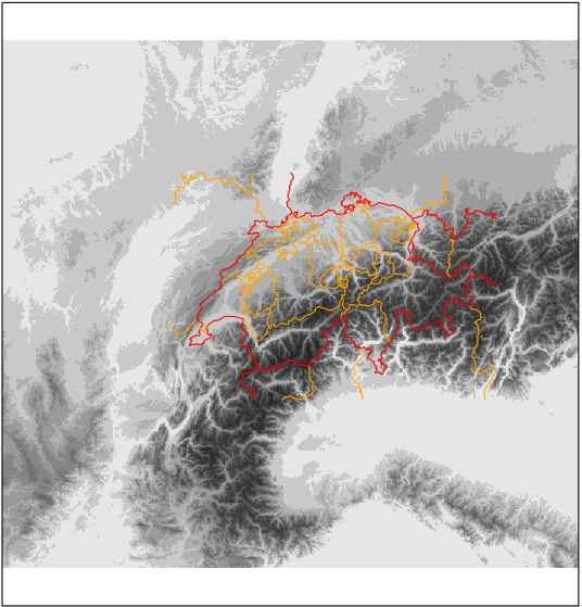
Let's start from the result. The following image shows what I'd like to achieve.
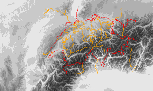
A cut-out of the resulting image.
Let's go to the R code. First, you have to load some libraries:
library(sp)
library(maps)
library(rgdal)
library(png)
library(raster)
Next, let's unzip the file downloaded from swisstopo and look for a file called VEC200_Com_Boundary.shp, which contains the polygons composing the swiss federal and cantonal borders. The content can be read like this:
ch<-readOGR(dsn="VEC200_Com_Boundary.shp",
layer="VEC200_Com_Boundary")
switzerland<-ch[ch$OBJVAL == "Landesgrenze",]
cantons<-ch[ch$OBJVAL == "Kantonsgrenze",]
Now we have to load the DEM data and assign to it the right projection description. The way you can reproject (with GDAL) the raw DEM to the swiss grid will be the subject for another post.
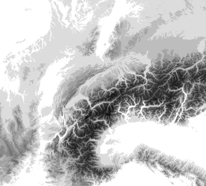
tdata<-readPNG("swiss_terrain.png");
terrain<-raster(tdata, 255000, 965000, -160000, 480000, crs="+proj=somerc
+lat_0=46.95240555555556 +lon_0=7.439583333333333 +k_0=1 +x_0=2600000
+y_0=1200000 +ellps=bessel +units=m +no_defs")
Finally, let's plot:
plot(terrain, col=gray(seq(0.1,0.9,length=255)), axis=FALSE, legend=FALSE,
frame.plot=FALSE, ann=FALSE, xaxt="n", yaxt="n")
plot(switzerland, col="red", add=TRUE, axis=FALSE, legend=FALSE,
frame.plot=FALSE, ann=FALSE, xaxt="n", yaxt="n")
plot(cantons, add=TRUE, col="orange", axis=FALSE, legend=FALSE,
frame.plot=FALSE, ann=FALSE, xaxt="n", yaxt="n")
Below you can find the png image of the terrain used in this example, as well as the final plot.